Arctic sea ice concentration with Clay embeddings and SAR
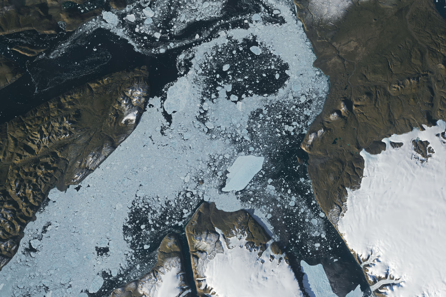
Testing whether embeddings from the Clay geospatial foundation model improve sea ice concentration mapping from Sentinel-1 SAR. Early results on a small sample favour plain backscatter statistics.
Employer: Sparkgeo (internal project)
When: 2026
Data: Sentinel-1 EW SAR (HH/HV), AMSR2 passive microwave, ERA5 reanalysis, Canadian Ice Service (CIS) and Danish Meteorological Institute (DMI) ice charts, via the AI4Arctic Sea Ice Challenge dataset
Methods: Clay v1.5 foundation model embeddings (frozen encoder), Random Forest, XGBoost
Stack: Python, PyTorch, Xarray, Rasterio, GeoPandas, GeoParquet, scikit-learn, XGBoost, AWS (S3, SageMaker), MLflow
Code: github.com/sparkgeo/arctic-showcase
Background
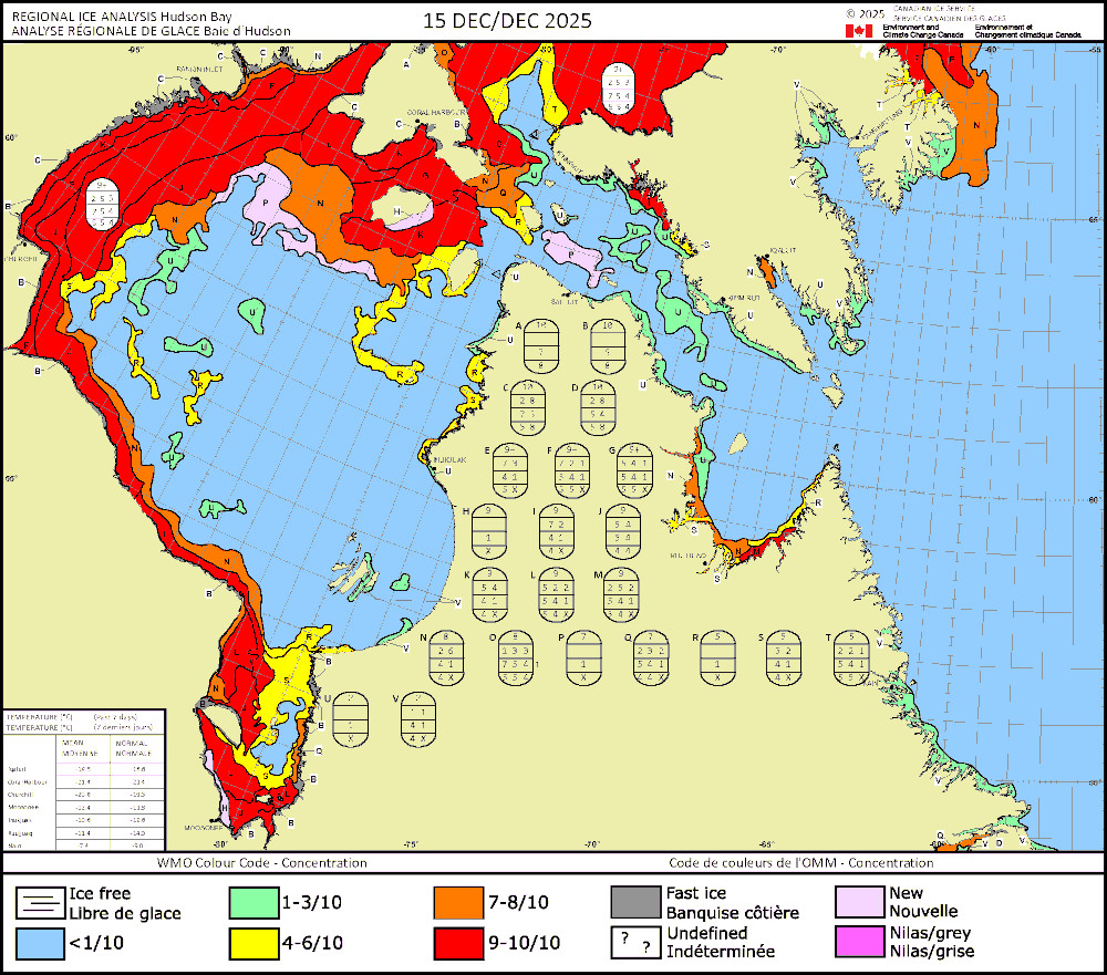
National ice services such as the Canadian Ice Service map sea ice concentration by hand: analysts interpret SAR images, draw polygons around areas of similar ice, and assign each a concentration in tenths. The charts are coarse, subjective, and take time to publish.
This project tests whether that can be automated on a much finer grid, using a geospatial foundation model. These are large models pre-trained on huge volumes of unlabelled Earth observation imagery, so they have already learned to represent texture, surface structure and spatial context. Training a sea ice model from scratch would need large amounts of high-quality labelled data. With a foundation model, the much smaller task is to learn how its representations map to ice concentration. The model is run once per scene, and lightweight classifiers can then be trained quickly on its output.
We used Clay v1.5, an open foundation model trained on imagery from several sensors, including Sentinel-1 SAR. Clay splits each image into small patches and turns each one into an embedding: a vector of 1024 numbers that summarizes what the patch looks like. One known risk: Clay’s Sentinel-1 training data came from a different acquisition mode and polarization pair (IW, VV/VH) from the Arctic imagery used here (EW, HH/HV), so its embeddings may not capture the features that matter most for sea ice.
The project classifies sea ice concentration into the 11 chart classes (0 to 10 tenths) on 320 m cells. That size is the footprint of one Clay patch at Sentinel-1 EW’s 40 m pixel spacing, so it is the model’s real effective resolution. Results are scored with R² on the 0 to 10 class values, the sea ice concentration metric of the AutoICE challenge the dataset was built for, so a prediction one class out counts as a smaller error than one five classes out.
The project was also designed to demonstrate a cloud-native data pipeline, with the source data and model outputs managed together in one catalogue. Hudson Bay in the 2025-26 ice season is the planned test region.
Approach
The plan has two tracks:
Modelling:
- train and evaluate on the AI4Arctic dataset, which bundles co-registered Sentinel-1, AMSR2, ERA5 and ice chart labels for 533 scenes.
- Each scene is cut into 256-pixel chips and passed through Clay unchanged (no fine-tuning), using a custom Clay sensor configuration for Sentinel-1 EW HH/HV with normalization statistics computed on the training scenes only. That gives an embedding for each 320 m patch, plus one for the whole chip.
- Each patch is labelled with the area-weighted average of the chart concentrations it overlaps, rounded down so a mixed patch is never labelled with more ice than it has.
- Random Forest and XGBoost classifiers then predict concentration from three feature sets: HH/HV backscatter statistics (the baseline), patch embeddings in place of the backscatter statistics, and patch plus chip embeddings.
- All three share the same AMSR2, ERA5, distance-to-land and incidence-angle inputs, so the comparison isolates what Clay adds. Fine-tuning Clay end to end is held back unless the frozen approach falls short on a validation split of the full dataset: R² below 0.8, or no gain over the baseline.
Cloud-native data and inference:
- Convert the 2025-26 Hudson Bay data to cloud-native formats (Cloud Optimized GeoTIFF, GeoParquet) and catalogue it with STAC.
- Run the trained model on new scenes, add the outputs to the same catalogue, and compare them with weekly CIS charts in a web map.
The modelling track is largely built: the training dataset pipeline (chipping, Clay encoding, per-patch features and labels, written to GeoParquet in S3), normalization statistics, and a first round of classifier training logged to MLflow. The inference track is in its early stages.
My contribution
- Designed the project and wrote the full technical plan: datasets, study area, model architecture, the feature sets, training strategy, and a phased implementation plan.
- Explored the AI4Arctic data formats to settle how the training data would be built.
- Supervised a co-op student who implemented most of the modelling track from that plan. I provided project context, continual guidance, and code review.
- Began implementing the inference pipeline.
Outcome
The project is currently paused. Full-scale runs haven’t been done yet, but are planned.
- About ten training scenes and one test scene were encoded. Validated within those scenes, all six combinations of feature set and classifier scored well (R² of 0.86 to 0.94), with the backscatter baseline highest. The validation data came from the same scenes as the training data, so these scores are optimistic.
- On one fully unseen scene, the best model (the baseline with XGBoost) reached R² = 0.385, an average error of about one concentration class. One scene is far too little to draw conclusions from.
- Two likely reasons the baseline led: Clay was pretrained on Sentinel-1 IW VV/VH imagery, not EW HH/HV over sea ice; and with about 1,000 embedding features, a Random Forest rarely considers the strong AMSR2 and ERA5 inputs at each split.
- Next steps: run the full dataset with whole-scene splits, add a linear probe and small neural network heads alongside the tree models, and fine-tune Clay if the full run meets the trigger above.